Mathematical Background

This section describes the mathematical background to the WDM wavelet transform.

Introduction

The Wilson-Daubechies-Meyer (WDM) wavelet basis is widely used for gravitational-wave (GW) data analysis. While far from being the only available choice, the WDM wavelets have several properties that make them well suited for this purpose: they are well separated in frequency which connects with the rest of GW data analysis which is almost exclusively done in the frequency domain; and they provide a uniform tiling in both time and frequency. The WDM wavelets were first introduced for GW data analysis in Ref. [1] (see also Ref. [2]) and have since been used in Coherent WaveBurst (CWB; see Refs. [3] and [4]).

This document is based on Refs. [1] and [2] with only a few minor changes in notation and conventions. The purpose of this document is to provide a complete, self-contained description of the WDM wavelet transform to accompany this JAX implementation, spelling out explicitly some details not discussed in the literature and correcting a few minor typos.

Fourier Transform Conventions

We use the following Fourier transform conventions:

(1)\[\tilde{X}(f) = \int_{-\infty}^{\infty} \mathrm{d}t\; \exp(-2\pi ift) x(t) ,\]

(2)\[x(t) = \int_{-\infty}^{\infty} \mathrm{d}f\; \exp(2\pi ift) \tilde{X}(f) .\]

For discrete signals, we use the following:

(3)\[\tilde{X}[\ell] = \delta t \sum_{k=0}^{N-1} x[k] \exp(-2\pi i \ell k / N) ,\]

(4)\[x[k] = \frac{1}{N\delta t} \sum_{\ell=-N/2}^{N/2-1} \tilde{X}[\ell] \exp(2\pi i\ell k/N) .\]

Meyer Window

The WDM wavelet transform is based on the Meyer window function, which is defined in the frequency domain by

(5)\[\begin{split}\tilde{M}(\omega) = \begin{cases} \sqrt{\frac{1}{\Delta\Omega}} & \text{if } |\omega| < A, \\ \sqrt{\frac{1}{\Delta\Omega}} \cos\left(\frac{\pi}{2}\nu_d\left(\frac{|\omega| - A}{B}\right)\right) & \text{if } A \leq |\omega| \leq A + B \\ 0 & \text{if } |\omega| > A + B \end{cases} ,\end{split}\]

where \(A>0\) and \(B>0\) control the shape of the window. The parameter \(A\) is the half-width of the flat-top response region and \(B\) is the width of the transition region; they satisfy \(2A + B = \Delta\Omega\), where \(\Delta\Omega\) is the total wavelet bandwidth. See Figure 1.

Figure 1 Top: the Meyer window function \(\tilde{M}(\omega)\) for different values of \(d\). Bottom: the time-domain window \(m(t)\), where \(\Delta T = \pi/\Delta\Omega\). The case \(d=4\) matches Fig.1 of Ref. [2]. Note how the wavelet is well localised in frequency (with compact support) but much less so in time.

The Meyer window function has the property that its square integrates to unity. To show this, first integrate over the flat-top part of the window (line 1), then let \(x=(\omega-A)/B\) (line 2), then use \(\cos^2 \theta = \frac{1+\cos(2\theta)}{2}\) (line 3), and finally use the symmetry \(\cos(\pi \nu_d(1-x))=\cos(\pi (1-\nu_d(x))) = \cos(\pi-\pi\nu_d(x)))= -\cos(\pi \nu_d(x))\) to set the remaining piece of the integral to zero (line 4):

(6)\[\begin{split}\begin{align} \int_{-\infty}^{\infty} \mathrm{d}\omega\; |\tilde{M}(\omega)|^2 &= \frac{2A+2\int_{A}^{A+B} \mathrm{d}\omega\; \cos^2\left(\frac{\pi}{2}\nu_d(\frac{\omega-A}{B})\right)}{2A+B} , \\ &= \frac{2A+2B \int_0^1 \mathrm{d}x\; \cos^2\left(\frac{\pi}{2}\nu_d(x)\right)}{2A+B} , \\ &= \frac{2A+2B \left(\frac{1}{2}+\frac{1}{2}\int_0^1\mathrm{d}x\; \cos\left(\pi\nu_d(x)\right)\right)}{2A+B} , \\ &= 1. \end{align}\end{split}\]

The Meyer function \(\tilde{M}(\omega)\) is implemented in WDM.code.utils.Meyer.Meyer().

Henceforth, we will work with frequency \(f\) instead of angular frequency \(\omega=2\pi f\). This fits with the rest of the GW data analysis community which generally uses \(f\).

For the wavelet transform, the frequency-domain window function is defined as

(7)\[\tilde{\Phi}(f) = \sqrt{2\pi} \tilde{M}(2\pi f) ,\]

and the corresponding time-domain window is

(8)\[\phi(t) = \int \mathrm{d}f \; \exp(2\pi i ft) \tilde{\Phi}(f)\]

These window functions are implemented in WDM.code.discrete_wavelet_transform.WDM.WDM_transform.build_frequency_domain_window() and WDM.code.discrete_wavelet_transform.WDM.WDM_transform.build_time_domain_window().

Unless otherwise stated, the default values \(A=\Delta\Omega/4\), \(B=\Delta\Omega/2\), and \(d=4\) will be used throughout the rest of this document.

WDM Wavelets

Consider a real-valued function of time \(x(t)\). The discretely sampled time series \(x[k]=x(t_k)\) is indexed by \(k\in\{0, 1, \ldots, N-1\}\) and evaluated at the sample times \(t_k=k\delta t\), where \(\delta t\) is the cadence and \(f_s = \frac{1}{\delta t}\) is the sampling frequency. The total duration of the time series is \(T=N\delta t\), and the Nyquist frequency is \(f_{\rm Ny}=\frac{1}{2\delta t}\). The frequency resolution is \(\delta f = \frac{1}{T}\).

The WDM wavelet transform represents the time series using \(N_f\) frequency slices of width \(\Delta F\) and \(N_t\) time slices of width \(\Delta T\);

(9)\[\Delta T = N_f \delta t ,\]

(10)\[\Delta F = \frac{1}{2 N_f \delta t} = \frac{N_t}{2T} .\]

There are \(N=N_t N_f\) cells, each with area \(\Delta T \Delta F = \frac{1}{2}\). These cells uniformly tile the time–frequency plane. We insist that both \(N_t\) and \(N_f\) are even. This implies that \(N\) is also even. Although not necessary, this simplifies some formulae and is not a significant limitation in practice.

The WDM wavelets \(g_{nm}(t)\) are constructed from the Meyer window function \(\phi\). The indices \(n\) and \(m\) label the time and frequency slices respectively. In the time-domain an orthonormal Wilson wavelet basis (Refs. [5] and [6]) can be defined as

(11)\[\begin{split}g_{nm}(t) = \begin{cases} \phi(t-2n\Delta T) & \mathrm{if}\;m=0 \\ \begin{cases} \sqrt{2} (-1)^{mn} \cos\left(\frac{\pi m t}{\Delta T}\right) \phi(t-n\Delta T) & \mathrm{if}\;n+m\;\mathrm{even}\\ \sqrt{2} \sin\left(\frac{\pi m t}{\Delta T}\right) \phi(t-n\Delta T) & \mathrm{if}\;n+m\;\mathrm{odd} \end{cases} & \mathrm{if}\;m>0 \end{cases} .\end{split}\]

Taking the Fourier transform, it is straightforward to show that the frequency-domain basis wavelets are given by

(12)\[\begin{split}\tilde{G}_{nm}(f) = \begin{cases} \exp(-4\pi i n f \Delta T) \tilde{\Phi}(f) & \mathrm{if}\;m=0 \\ \frac{1}{\sqrt{2}}\exp(-2\pi i n f \Delta T) \left( C_{nm}\tilde{\Phi}(f+m\Delta F) +C^*_{nm}\tilde{\Phi}(f-m\Delta F) \right) & \mathrm{if}\;m>0 \end{cases} ,\end{split}\]

where

(13)\[\begin{split}C_{nm} = \begin{cases} 1 & \mathrm{if}\;n+m\;\mathrm{even} \\ i & \mathrm{if}\;n+m\;\mathrm{odd} \end{cases} .\end{split}\]

If the time index is allowed to vary in the range \(n\in\{0,1,\ldots,N_t-1\}\) then the wavelet basis covers the full range of the time series. However, in order to cover the full frequency range (up to the Nyquist frequency) the frequency index must be allowed to vary in the range \(m\in\{0,1,\ldots, N_f\}\) (including \(N_f\)). The \(m=N_f\) wavelets have support below the Nyquist frequency; see Figure 2. The case \(m=N_f\) is handled as a special case using the following formulae:

(14)\[g_{nN_f}(t) = \cos(2\pi f_{\rm Ny}[t-2n\Delta T]) \phi(t-2n\Delta T),\]

(15)\[\tilde{G}_{nN_f}(f) = \frac{1}{2} \exp(-4\pi i n f \Delta T) \left( \tilde{\Phi}(f-f_{\rm Ny}) + \tilde{\Phi}(f+f_{\rm Ny}) \right) .\]

Notice that for most of the wavelets the index \(n\) shifts the wavelets by integer multiples of \(\Delta T\) in time. However, for \(m=0\) and \(m=N_f\) it shifts them by integer multiples of \(2\Delta T\).

The WDM wavelets are plotted in the frequency domain in Figure 2.

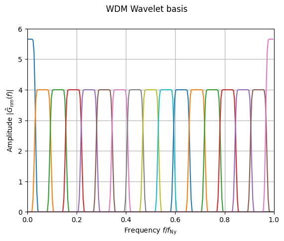
Figure 2 The \(d=4\) WDM wavelets \(|\tilde{G}_{nm}(f)|\) plotted in the frequency domain for \(m=0, 1, 2,\ldots,N_f\). Wavelets computed using \(N_f=16\) are shown to match Fig.2 of Ref. [1].

As defined, the index \(m\) takes on both values 0 and \(N_f\). However, these two cases can be conveniently grouped together. Because of the \(2\Delta T\) time shift, only half of the \(n\) range is needed for these \(m\) indices; therefore, we redefine \(G_{n0}(f):=G_{nN_f}(f)\) when \(n\geq N_t/2\). With this choice, the index ranges \(n\in\{0,1,\ldots,N_t-1\}\) and \(m\in\{0,1,\ldots,N_f-1\}\) cover the entire time-frequency plane; see Figure 5. The central time and frequency of the wavelet \(g_{nm}(t)\) are given by

(16)\[\begin{split}t_{nm} = \begin{cases} 2 n \Delta T & \mathrm{if}\;m=0 \\ n \Delta T & \mathrm{if}\;m>0 \end{cases} \,,\end{split}\]

(17)\[\begin{split}f_{nm} = \begin{cases} \begin{cases}0&\mathrm{if}\;n<N_t/2\\ f_{\rm Ny}&\mathrm{if}\,n\geq N_t/2\end{cases} & \mathrm{if}\;m=0 \\ m \Delta F & \mathrm{if}\;m>0 \end{cases} \,.\end{split}\]

These expressions are implemented in WDM.code.discrete_wavelet_transform.WDM.WDM_transform.wavelet_central_time_frequency().

Examples of the WDM wavelets with \(N=512\), \(N_f=16\), and \(\delta t=1\) are shown in Figure 3, Figure 4, and Figure 5. Notice that the WDM wavelets are well localised in frequency but much less so in time.

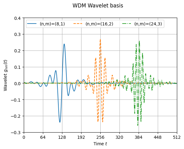
Figure 3 The time-domain WDM wavelets \(g_{nm}(t)\) for selected values of \(n\) and \(m\).

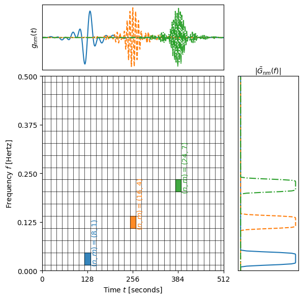
Figure 4 The WDM wavelets plotted in both time (top) and frequency (right) domain for selected \(n\) and \(m\). The main plot shows a time-frequency grid shaded to indicate where the wavelets have support.

Figure 5 Animated version of Figure 4 looping through all the wavelets. Notice in particular the behaviour of the wavelets for \(m=0\).

The discretely sampled WDM wavelets have the following orthonormality properties:

(18)\[\delta t \sum_{k=0}^{N-1} g_{nm}[k] g_{n'm'}[k] = \delta_{nn'} \delta_{mm'} .\]

(19)\[\delta f \sum_{\ell=-N/2}^{N/2-1} \tilde{G}_{nm}[\ell] \tilde{G}^*_{n'm'}[\ell] = \delta_{nn'} \delta_{mm'} .\]

The frequency-domain WDM wavelets \(\tilde{G}_{nm}(f)\) are implemented in WDM.code.discrete_wavelet_transform.WDM.WDM_transform.Gnm() or WDM.code.discrete_wavelet_transform.WDM.WDM_transform.Gnm_basis().

The time-domain WDM wavelets \(g_{nm}(t)\) are implemented in WDM.code.discrete_wavelet_transform.WDM.WDM_transform.gnm() or WDM.code.discrete_wavelet_transform.WDM.WDM_transform.gnm_basis().

The Discrete Wavelet Transform

The WDM wavelets form a complete orthonormal basis for real-valued, discretely sampled time series,

(20)\[x[k] = \sum_{n=0}^{N_t-1} \sum_{m=0}^{N_f-1} w_{nm} g_{nm}[k] .\]

Here, \(x[k]\) is the input time series, \(w_{nm}\) are the wavelet coefficients, and \(g_{nm}[k]\) are the WDM wavelet basis functions.

An expression for the wavelet coefficients \(w_{nm}\) can be derived by multiplying both sides of this equation by \(\delta t \, g_{n'm'}[k]\), summing over \(k\), and using the above orthonormality property to obtain

(21)\[w_{nm} = \delta t\sum_{k=0}^{N-1} x[k] g_{nm}[k] .\]

This is the exact expression for the forward wavelet transform which transforms from the time domain to the time-frequency domain.

This exact wavelet transform is implemented in WDM.code.discrete_wavelet_transform.WDM.WDM_transform.forward_transform_exact().

The exact form of the wavelet transform described above and with the double sum evaluated explicitly is slow to evaluate. The rest of this section describes several alternative formulations of the wavelet transform leading eventually to a fast implementation based on the FFT of the time series data.

One way to speed up the wavelet transform is to notice that the WDM wavelets are (approximately) localised in time. Therefore, we don’t need to sum over all values of \(k\) when evaluating the wavelet coefficients. The sum can be truncated to a window of length \(K=2qN_f\) without significant loss of accuracy. The truncation parameter \(1\leq q\leq N_t/2\) is a positive integer that controls the length of the window. The truncated window must be centered at the time where the wavelet amplitude is largest. The truncated wavelet transform is given by

(22)\[w_{n0} = \delta t\sum_{k=-K/2}^{K/2-1} g_{n0}[k + 2 n N_f] x[k + 2 n N_f] ,\]

(23)\[w_{nm} = \delta t\sum_{k=-K/2}^{K/2-1} g_{nm}[k + n N_f] x[k + n N_f] \quad \mathrm{for} \; m>0.\]

In expressions such as these, indices that are out of bounds of the array are to be understood as wrapping around circularly; i.e. \(x[-1] = x[N-1]\) and \(x[N] = x[0]\).

This form of the truncated wavelet transform is implemented in WDM.code.discrete_wavelet_transform.WDM.WDM_transform.forward_transform_truncated().

Smaller values of \(q\) yield faster but less accurate wavelet transforms. The accuracy of this truncated wavelet transform is explored in the example notebook Exploring the accuracy of the truncated wavelet transform.

The truncated wavelet transform can be rewritten in terms of the window function \(\phi[k]\);

(24)\[\begin{split}w_{n0} = \delta t \begin{cases} \sum_{k=-K/2}^{K/2-1} x[k+2nN_f]\phi[k] & \mathrm{if}\;n<N_t/2 \\ \sum_{k=-K/2}^{K/2-1} (-1)^k x[k+2nN_f]\phi[k] & \mathrm{if}\;n\geq N_t/2 \\ \end{cases} ,\end{split}\]

(25)\[w_{nm} = \sqrt{2}\delta t \, \mathrm{Re} \sum_{k=-K/2}^{K/2-1} C^*_{nm} \exp\left(\frac{i\pi km}{N_f}\right) x[k+nN_f] \phi[k] \quad \mathrm{for}\; m>0.\]

To derive these expressions, substitute the definitions of the time-domain wavelets \(g_{nm}[k]\) in Eq.9 (and the special case in Eq.12) into the truncated expressions for the wavelet coefficients in Eqs.22 and 23.

This form of the truncated window wavelet transform using \(\phi[k]\) is implemented in WDM.code.discrete_wavelet_transform.WDM.WDM_transform.forward_transform_truncated_window().

The need to handle the \(m=0\) terms separately can slow down the wavelet transform. This is often unnecessary as the lowest and highest frequency parts of the signal are often not needed. Therefore, by default the WDM_transform class that implements these transformations will not use the formulae for the special case \(m=0\) and therefore miscalculates these coefficients. If the \(m=0\) coefficients are needed, then the class should be initialised with the keyword argument calc_m0=True. The effect of getting the \(m=0\) coefficients wrong on the signal reconstructed from the wavelet coefficients is explored in the example notebook m=0 Wavelet Coefficients.

The wavelet transform can be considerably sped up by exploiting the fast Fourier transform (FFT) algorithm. Let us define

(26)\[X_n[j] = \sum_{k=-K/2}^{K/2-1} \exp(2\pi i kj/K) x[nN_f+k] \phi[k] .\]

This can be thought of as a short FFT. (Although, with our conventions it’s actually an inverse FFT.) The data is first split into \(N_t\) overlapping segments of length \(K\), each segment is multiplied by the window function \(\phi[k]\) and the (inverse) FFT is applied to each segment.

The short FFT to calculate \(X_n[j]\) is implemented in WDM.code.discrete_wavelet_transform.WDM.WDM_transform.short_fft().

The expression for the wavelet coefficients in Eq.23 can be rewritten using this short FFT downsampled to extract every \(q^{\rm th}\) coefficient,

(27)\[w_{nm} = \sqrt{2} \delta t \, \mathrm{Re}\, C_{nm}^* X_n[mq] \quad \mathrm{for}\; m>0.\]

This formula for the wavelet coefficients only holds for \(m>0\). If the \(m=0\) terms are required they are calculated using the truncated window expressions above (Eq.22).

This short FFT form of the wavelet transform is implemented in WDM.code.discrete_wavelet_transform.WDM.WDM_transform.forward_transform_short_fft().

This is pretty fast. But it turns out that a further speed up is possible if instead we perform the full FFT on the original time series, rather than the short FFT. The reason this is faster is to do with the fact that our chosen WDM wavelets are better localised in the frequency domain than in the time domain (see discussion in Ref. [1]). This also has the benefit of not introducing any truncation errors in the forward wavelet transform because the WDM wavelets have compact support in frequency.

To derive the FFT expression for the wavelet transform start from the definition of the wavelet coefficients \(w_{nm}\) in Eq.19 and use Parseval’s theorem (discrete form) to write them as

(28)\[w_{nm} = \frac{1}{T} \sum_{\ell=-N/2}^{N/2-1} \tilde{X}[\ell] \tilde{G}_{nm}[\ell] .\]

Now use the expression for \(\tilde{G}_{nm}(f)\) in Eq.12 evaluated at the discrete FFT frequencies \(f_\ell = \ell \delta f\) to write this as

(29)\[w_{nm} = \frac{1}{\sqrt{2}T} \sum_{\ell=-N/2}^{N/2-1} \tilde{X}[\ell] \exp(2\pi in\ell /N_t) \left( C_{nm}^*\tilde{\Phi}[\ell+mN_t/2] + C_{nm}\tilde{\Phi}[\ell-mN_t/2] \right) .\]

Reindexing the first term using \(\ell'=\ell+mN_t/2\) gives

(30)\[\mathrm{first}\;\mathrm{term} = \frac{(-1)^{nm}}{\sqrt{2}T} \sum_{\ell'=-N/2}^{N/2-1} \exp(2\pi i n \ell' / N_t) \tilde{X}[\ell'-mN_t/2] \tilde{\Phi}[\ell'] .\]

Reindexing the second term using \(\ell'=\ell-mN_t/2\) and using the fact that freqency-domain window is real and and even (\(\tilde{\Phi}[-\ell]=\tilde{\Phi}[-\ell]\) and \(\tilde{\Phi}[\ell]\in\mathbb{R}\)), and the fact that the original time series is real (\(x[k]\in\mathbb{R}\)) means that it’s Fourier transform has Hermitian symmetry (\(X[-\ell]=X[\ell]^*\)), gives

(31)\[\mathrm{second}\;\mathrm{term} = \frac{(-1)^{nm}}{\sqrt{2}T} \sum_{\ell'=-N/2}^{N/2-1} \exp(-2\pi i n \ell' / N_t) \tilde{X}^*[\ell'-mN_t/2] \tilde{\Phi}[\ell'] .\]

Putting these together and dropping the prime on the index gives

(32)\[w_{nm} = \frac{\sqrt{2}}{T} (-1)^{nm} \,\mathrm{Re}\, C_{nm}^* \sum_{\ell'=-N/2}^{N/2-1} \exp\left(2\pi i n \ell'/N_t\right) \tilde{X}[\ell-m N_t/2] \tilde{\Phi}[\ell] .\]

The fact that the frequency-domain window has compact support means this sum can be truncated without any loss of accuracy,

(33)\[w_{nm} = \frac{\sqrt{2}}{T} (-1)^{nm} \,\mathrm{Re}\, C_{nm}^* \sum_{\ell'=-N_t/2}^{N_t/2-1} \exp\left(2\pi i n \ell'/N_t\right) \tilde{X}[\ell-m N_t/2] \tilde{\Phi}[\ell] .\]

The sum in this expression can be computed efficiently using an FFT; letting

(34)\[x_m[n] = \sum_{\ell'=-N_t/2}^{N_t/2-1} \exp\left(2\pi i n \ell'/N_t\right) \tilde{X}[\ell-m N_t/2] \tilde{\Phi}[\ell] ,\]

we arrive at our final expression for the wavelet coefficients,

(35)\[w_{nm} = \frac{\sqrt{2}}{T} (-1)^{nm} \,\mathrm{Re}\, C_{nm}^* x_m[n] .\]

This is our final FFT form of the wavelet transform and is implemented in WDM.code.discrete_wavelet_transform.WDM.WDM_transform.forward_transform_fft().

Again, this FFT expression for the wavelet coefficients only holds for \(m>0\). If the \(m=0\) terms are required they are calculated using the truncated window expressions above (Eq.22).

This FFT form of the wavelet transform is the fast version intended for production use. This method is also vectorised to allow for efficient batch processing of multiple time series.

The speed of all the implementations discussed here are compared in the example notebook Benchmarking.

Units

The time-domain wavelets have dimension \(\big[g_{nm}\big]=\sqrt{1/\mathrm{time}}\) and the frequency-domain wavelets have dimension \(\big[\tilde{G}_{nm}\big]=\sqrt{\mathrm{time}}\).

If the time series \(x(t_k)=x[k]\) has dimension \(\big[x\big]=\alpha\) then the wavelet coefficients have dimension \(\big[w_{nm}\big]=\alpha\sqrt{\mathrm{time}}\).

Glossary

• \(t\): Time (e.g. seconds).

• \(f\): Frequency (e.g. Hertz).

• \(\omega\): Angular frequency (radians per unit time). Defined as \(\omega=2\pi f\).

• \(\delta t\): Time series cadence (time units). Named dt in WDM_transform.

• \(f_{\rm Ny}\): Nyquist frequency, or the maximum frequency (frequency units). Defined as \(f_{\rm Ny}=\frac{1}{2 \delta t}\). Named f_Ny in WDM_transform.

• \(f_{s}\): Sampling frequency (frequency units). Defined as \(f_{s}=\frac{1}{\delta t}\). Named f_s in WDM_transform.

• \(A\): Width of flat-top response in the Meyer window (radians per unit time). Named A in WDM_transform.

• \(B\): Width of transition region in the Meyer window (radians per unit time). Named B in WDM_transform.

• \(\Delta\Omega\): Angular frequency resolution of the wavelets (radians per unit time). Satisfies \(\Delta\Omega = 2A + B\). Named dOmega in WDM_transform.

• \(\Delta F\): Frequency resolution of the wavelets (frequency units). Satisfies \(\Delta F = \frac{\Delta\Omega}{2\pi}\). Named dF in WDM_transform.

• \(\Delta T\): Time resolution of the wavelets (time units). Satisfies \(\Delta T \Delta F= \frac{1}{2}\). Named dT in WDM_transform.

• \(d\): Steepness parameter for the Meyer window. Named d in WDM_transform.

• \(q\): Truncation parameter for the freqency-domain window. Named q in WDM_transform.

• \(N_f\): Number of frequency bands for the wavelets. Named Nf in WDM_transform.

• \(N_t\): Number of time bands for the wavelets, must be even. Named Nt in WDM_transform.

• \(N\): Number of points in the time series. Satisfies \(N = N_t N_f\). Named N in WDM_transform.

• \(T\): Duration of the time series (time units). Satisfies \(T = N \delta t\). Named T in WDM_transform.

• \(n\): Time index for the wavelets. In the range \(n\in\{0,1,\ldots, N_t-1\}\).

• \(m\): Frequency index for the wavelets. In the range \(m\in\{0,1,\ldots, N_f-1\}\). The \(m=0\) terms store both the zero frequency (\(f\approx 0\)) and the Nyquist frequency (\(f\approx f_{\rm Ny}\)) terms.

• \(x[k]\): Time series data, where \(k\in\{0,1,\ldots,N-1\}\) indexes the time.

• \(\tilde{\Phi}(f)\): Frequency-domain window function, \(\tilde{\Phi}(f)=\sqrt{2\pi}\tilde{M}(2\pi f)\).

• \(\phi(t)\): Time-domain Meyer window, defined as the inverse Fourier transform of \(\tilde{\Phi}(\omega)\).

• \(\tilde{G}_{nm}(f)\): Frequency-domain WDM wavelet.

• \(g_{nm}(t)\): Time-domain WDM wavelet, defined as the inverse Fourier transform of \(\tilde{G}_{nm}(\omega)\).

• \(w_{nm}\): The wavelet coefficients.

References

[1] (1,2,3,4)

V. Necula, S. Klimenko & G. Mitselmakher, Transient analysis with fast Wilson-Daubechies time-frequency transform, Journal of Physics: Conference Series 363 012032, 2012. DOI 10.1088/1742-6596/363/1/012032

[2] (1,2,3)

N. J. Cornish, Time-Frequency Analysis of Gravitational Wave Data, Physical Review D 102 124038, 2020. arXiv:2009.00043

[3]

S. Klimenko, S. Mohanty, M. Rakhmanov & G. Mitselmakher, Constraint likelihood analysis for a network of gravitational wave detectors, Physical Review D 72, 122002, 2005. arXiv:gr-qc/0508068

[4]

S. Klimenko et al., Method for detection and reconstruction of gravitational wave transients with networks of advanced detectors, Physical Review D 93, 042004, 2016. arXiv:1511.05999

[5]

K. G. Wilson, Generalized Wannier functions, preprint, Cornell University. link

[6]

I. Daubechies, S. Jaffard & J. L. Journé, A simple Wilson orthonormal basis with exponential decay, SIAM Journal on Mathematical Analysis, 22, 2, 554–572, 1991. DOI 10.1137/0522035

Appendices

Normalised Incomplete Beta Function

The WDM wavelets use the normalised incomplete beta function, \(\nu_d(x)\),

(36)\[\nu_d(x) = \frac{ \int_0^x \mathrm{d}t \, t^{d-1} (1 - t)^{d-1} } { \int_0^1 \mathrm{d}t \, t^{d-1} (1 - t)^{d-1} } , \quad \mathrm{for}\; 0\leq x\leq 1.\]

This acts as a smooth transition function (or compact sigmoid-like function) from 0 to 1. The parameter \(d\) controls the steepness of the transition; see Figure 6.

The details of this function are actually not very important; any function that increases smoothly \(\nu(0)=0\) to \(\nu(1)=1\) and has the symmetry \(\nu(1-x)=1-\nu(x)\) will produce sensible wavelets.

The function \(\nu_d(x)\) is implemented in WDM.code.utils.Meyer.nu_d().

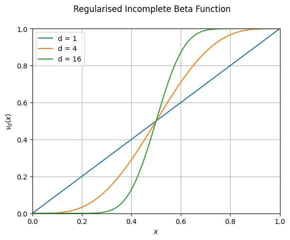
Figure 6 The normalised incomplete beta function \(\nu_d(x)\) for several values of \(d\).