Mathematical Background

This section describes the mathematical background to the fast wavelet transform of harmonic-based GW waveform models.

Introduction

Gravitational waveform models are usually constructed in either the time domain (TD; \(h_+(t)\), \(h_\times(t)\)) or the frequency domain (FD; \(\tilde{h}_+(f)\), \(\tilde{h}_\times(f)\)). If gravitational wave data analysis is to be performed in the time-frequency domain (TFD) then it is also necessary to transform our models into this TFD.

This document describes a fast method for transforming harmonic-based waveforms from either the time to the time-frequency domain (TD \(\rightarrow\) TFD) of from the frequency to the time-frequency domain (FD \(\rightarrow\) TFD). These fast transforms rely on expanding the waveform phase (e.g.as a function of time) in each harmonic. This requires that the frequency is slowly varying over the scale of the wavelets. These fast transforms have some similarities with the stationary phase approximation which is used to compute the Fourier transform between the time and frequency domains.

The next section starts by reviewing the Wilson-Daubechies-Meyer (WDM) wavelets which are used throughout as a basis for the TFD. The fast TD \(\rightarrow\) TFD and FD \(\rightarrow\) TFD transforms are described in subsequent two sections respectively.

WDM Wavelets

The WDM family of wavelets are implemented in the WDM_GW_wavelets package (WDM docs); see also Ref. [1] and Ref. [2]. The basis wavelets can be written as

(1)\[\begin{split}g_{nm}(t) = \begin{cases} \sqrt{2} \cos\left(2\pi m [t-n\Delta T] \Delta F\right) \phi(t-n\Delta T) & \mathrm{if}\;n+m\;\mathrm{even} \\ \sqrt{2} (-1)^{nm} \sin\left(2\pi m [t-n\Delta T] \Delta F\right) \phi(t-n\Delta T) & \mathrm{if}\;n+m\;\mathrm{odd} \end{cases} ,\end{split}\]

where \(\phi(t)\) is a universal window function. The \(n\) index shifts the central time \(n\Delta T\) of the wavelet while the \(m\) index shifts the central frequency \(m\Delta F\). The wavelet time and frequency resolutions satisfy \(\Delta F \Delta T=1/2\). These expressions hold for all values of \(n=0,1,\ldots, N_{t}-1\) but only for non-zero values of \(m=1,2,\ldots, N_{f}-1\); the \(m=0\) wavelets store the zero and Nyquist frequency components of the signal and have to be handled separately. It will also be necessary to use the dual WDM wavelet basis;

(2)\[\begin{split}\hat{g}_{nm}(t) = \begin{cases} \sqrt{2} \sin\left(2\pi m [t-n\Delta T] \Delta F\right) \phi(t-n\Delta T) & \mathrm{if}\;n+m\;\mathrm{even} \\ \sqrt{2} (-1)^{nm} \cos\left(2\pi m [t-n\Delta T] \Delta F\right) \phi(t-n\Delta T) & \mathrm{if}\;n+m\;\mathrm{odd} \\ \end{cases}.\end{split}\]

The two bases are related by a time shift \(\Delta T/2\) and span exactly the same space; see the discussion in Ref. [1].

Fast Wavelet Transform (TD \(\rightarrow\) TFD)

Suppose we are given a waveform in the TD defined in terms of its amplitude \(A(t)\) and phase \(\Phi(t)\),

(3)\[h(t) \equiv h^+(t)-ih^\times(t) = A(t) \exp\big(i \Phi(t)\big) .\]

Suppose the amplitude and frequency (\(2\pi f(t) = \mathrm{d}\Phi/\mathrm{d}t\)) change slowly with time; i.e.they change by a small amount over the wavelet timescale \(\Delta T\). This is a signal harmonic and a waveform may contain a sum of such harmonics. This is what is meant above by “harmonic-based waveform”.

The wavelet coefficients are defined as

(4)\[w_{nm} \equiv w^+_{nm} -i w^\times_{nm} = \int_{-\infty}^\infty\mathrm{d}t\;h(t)g_{nm}(t).\]

Strictly speaking the wavelet coefficients for the discrete wavelet transform involve a sum (not an integral) over the time series \(t_i=i\delta t\) for \(i=0,1,\ldots, N-1\), where \(N=N_t N_f\). However, most of our expressions will be unaffected by changing from a sum to an integral so we continue to use this nicer notation.

The basis wavelet \(g_{nm}(t)\) is well localised around the time \(t\sim t_n\pm\Delta T\). Motivated by the fact that the amplitude and frequency are slowly varying, we Taylor expand these quantities about \(t_n\);

(5)\[A(t) = A(t_n) + \mathcal{O}(t-t_n)\]

(6)\[\Phi(t) = \Phi(t_n) + 2\pi f(t_n) (t-t_n) + \pi \dot{f}(t_n) (t-t_n)^2 + \mathcal{O}\big((t-t_n)^3\big)\]

where

(7)\[f(t) = \frac{1}{2\pi}\frac{\mathrm{d}}{\mathrm{d}t}\Phi(t)\]

and

(8)\[\dot{f}(t) = \frac{1}{2\pi}\frac{\mathrm{d}^2}{\mathrm{d}t^2}\Phi(t)\]

and so on for higher derivatives.

It is important that the amplitude is expanded only to zeroth order (as shown above) but the phase can be expanded to any order depending on the accuracy needed. Substituting these expansions into the definition of the wavelet coefficients gives

(9)\[w_{nm} = A(t_n)\exp\big(i\Phi(t_n)\big)\left(c_{nm}\big(f(t_n),\dot{f}(t_n), \ldots\big) + i s_{nm}\big(f(t_n),\dot{f}(t_n), \ldots\big) \right),\]

where we have defined

(10)\[c_{nm}(f, \dot{f}, \ldots) = \int\mathrm{d}t\;\cos X_n(f, \dot{f}, \ldots) g_{nm}(t) ,\]

(11)\[s_{nm}(f, \dot{f}, \ldots) = \int\mathrm{d}t\;\sin X_n(f, \dot{f}, \ldots) g_{nm}(t) ,\]

where

(12)\[X_n(f,\dot{f},\ldots) = 2\pi(t-n\Delta T)f+\pi(t-n\Delta T)^2\dot{f} + \ldots \quad .\]

It will also be necessary to use the dual coefficients \(\hat{c}_{nm}\) and \(\hat{s}_{nm}\) defined similarly using \(\hat{g}_{nm}\).

Our approach will be to evaluate the waveform amplitude (\(A(t_n)\)), phase (\(\Phi(t_n)\)), and as many phase derivatives (\(f(t_n)\), \(\dot{f}(t_n)\), …) as required at the wavelet times \(t_n\); note, that this is much sparser grid of times than that of the original time series. We will then evaluate the quantities \(c_{nm}\) and \(s_{nm}\) by interpolating these as functions of \(f\), \(\dot{f}\), … over a precomputed grid of points. Finally, the wavelet coefficients will be obtained using the above expression for \(w_{nm}\). By pre-computing and interpolating \(c_{nm}\) and \(s_{nm}\) this approach amortizes the cost of evaluating the oscillatory integrals over time involved in transforming to the TFD.

The interpolation of the \(c_{nm}\) and \(s_{nm}\) coefficients is greatly aided by the following observations: first, to a good approximation the coefficients only depend on the parity of the index \(n\); and second, these quantities have a shift symmetry in frequency which relates the coefficients at a frequency \(f\) to the coefficients at \(f+2\Delta F\). The importance of the first observation is that it means it only necessary to interpolate one row of the coefficient matrices. The importance of the second observation is that it is only necessary to interpolate over a narrow range of frequencies and the coefficients at any frequency can then be obtained by shifting by even multiples of \(\Delta F\). We now describe these two observations in turn.

OBSERVATION 1:

This observation means the coefficients only depend on the parity of the index \(n\). This can be made precise using the following results derived in appendix A that relate the coefficients at a general \(n\) to the coefficients at a fixed even index \(\mathcal{N}\);

(13)\[\begin{split}c_{nm}(f, \dot{f},\ldots) = \begin{cases} c_{\mathcal{N}m}(f, \dot{f},\ldots) & \mathrm{if}\;n\;\mathrm{is}\;\mathrm{even} \\ \hat{c}_{\mathcal{N}m}(f, \dot{f},\ldots) & \mathrm{if}\;n\;\mathrm{is}\;\mathrm{odd} \end{cases} ,\end{split}\]

(14)\[\begin{split}s_{nm}(f, \dot{f},\ldots) = \begin{cases} s_{\mathcal{N}m}(f, \dot{f},\ldots) & \mathrm{if}\;n\;\mathrm{is}\;\mathrm{even} \\ \hat{s}_{\mathcal{N}m}(f, \dot{f},\ldots) & \mathrm{if}\;n\;\mathrm{is}\;\mathrm{odd} \end{cases} .\end{split}\]

If we use these results, then we see that it is only necessary to compute the coefficients \(c_{nm}\) and \(s_{nm}\) for a single value of the index \(n=\mathcal{N}\) (provided we also compute \(\hat{c}_{\mathcal{N}m}\) and \(\hat{s}_{\mathcal{N}m}\)) and all other coefficients with general \(n\) can be obtained from just these.

Unfortunately, these time-shift equations do not hold exactly for the discrete wavelet transform. These expressions were derived in Appendix A using the integral expressions (over \(t\in(-\infty,\infty)\)) for the wavelet coefficients. When using finite sums, the periodic boundary conditions spoil the time-translation properties of the wavelets used in the derivation. The result is that these expressions are only valid for wavelets localised away from the beginning or end of the time range. This is illustrated in Figure 1. For this reason, we choose \(\mathcal{N}\) to be somewhere nicely in the middle of the time series.

All numerical results shown here were obtained with a time series duration \(T=2^{16}\,\mathrm{s}\) and sampling frequency of \(1/\delta t = 1\,\mathrm{Hz}\). The basis wavelets have \(N_t=512\), \(q=16\), \(d=4\) and \(A=\pi /512\,\mathrm{rad}\,\mathrm{s}^{-1}\); these choices lead to \(N_f=128\) and time-frequency resolutions \(\Delta T=128\,\mathrm{s}\) and \(\Delta F=256^{-1}\,\mathrm{Hz}\). It will be convenient to fix a reference frequency, this is taken to be half the Nyquist frequency, or \(f_{\rm ref}=N_f\Delta F/2\).

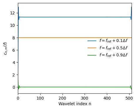
Figure 1 This plot shows the coefficient \(c_{nm}(f)\) for several value of \(f\) (\(\dot{f}\) and all higher derivatives are set to zero) for a fixed value of \(m=N_f/2\) plotted as a function of the index \(n\) for even values (i.e.\(n=0,2,4,\ldots, N_t-2\)). To an good approximation the \(c_{nm}\) coefficients do not depend on the index \(n\); this approximation breaks down near the ends of the time series where the periodic boundaries are significant.

OBSERVATION 2:

This observation allows the coefficients at a frequency shifted by an even multiple of the wavelet resolution \(\Delta F\) to be written in terms of the coefficients evaluated at the reference frequency. This can be made precise using the following results derived in appendix B that relate the coefficients at frequency \(f+2z\Delta F\) to the coefficients at frequency \(f\) for any integer \(z\);

(15)\[c_{nm}(f+2z\Delta F) \!=\! \frac{1}{2} \left( c_{n(m-2z)}(f) + c_{n(m+2z)}(f) + (-1)^{n+m} \hat{s}_{n(m-2z)}(f) - (-1)^{n+m} \hat{s}_{n(m+2z)}(f) \right) ,\]

(16)\[s_{nm}(f+2z\Delta F) \!=\! \frac{1}{2} \left( s_{n(m-2z)}(f) + s_{n(m+2z)}(f) - (-1)^{n+m} \hat{c}_{n(m-2z)}(f) + (-1)^{n+m} \hat{c}_{n(m+2z)}(f) \right) .\]

Using these results, we see that it is only necessary to interpolate the coefficients over a narrow range \(f_{\rm ref}\leq f<f_{\rm ref}+2\Delta F\) in frequency. We choose the fixed reference frequency \(f_{\rm ref}\) to be somewhere nicely in the middle of the bandwidth of interest. A general frequency \(f\) can be written as the sum of a piece in this ranges \(F(f)\) and a shift by an even multiple \(2z(f)\) of \(\Delta F\);

(17)\[f = F(f) + 2z(f) \Delta F ,\]

where

(18)\[F(f) = \big(f-f_{\rm ref}\big)\,\mathrm{mod}\,(2\Delta F) + f_{\rm ref}\]

and

(19)\[z(f) = \left\lfloor \frac{f-f_{\rm ref}}{2\Delta F}\right\rfloor .\]

An example of the data to be interpolated is shown in Figure 2.

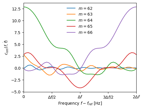
Figure 2 An example of the coefficient data to be interpolated. Here the coefficients \(c_{nm}(f,\dot{f})\) are plotted as a function of frequency in the range \(f_{\rm ref}<f<f_{\rm ref}+2\Delta F\). The time index is fixed to \(n=N_t/2\) and results are shown for several values of \(m\) close to the reference frequency. The frequency derivative is fixed to \(\dot{f}=10^{-5}\,\mathrm{Hz}\,\mathrm{s}^{-1}\).

We are now in a position to describe the fast wavelet transform (TD \(\rightarrow\) TFD). The following steps must be performed once to set up the transformer:

• Fix the properties of the times series. This involves choosing the time series parameters: e.g.duration \(T\), sampling frequency \(1/\delta t\), number of samples \(N\), etc.

• Fix the wavelet basis. This involves choosing the wavelet parameters: e.g. the time-frequency resolution \(\Delta T\) and \(\Delta F\) and the shape parameters of the mother wavelet \(A\), \(B\), \(q\) and \(d\).

• Choose how many terms to include in the phase expansion, i.e. how many frequency derivatives to interpolate over. This choice is related to the wavelet resolution \(\Delta T\) and maximum expected chirp rate of the waveform with faster chirps and finer resolutions generally requiring more derivatives. By default we will include only the \(f\) term.

• Fix values the reference values for \(\mathcal{N}\) and \(f_{\rm ref}=\mathcal{M}\Delta F\). By default we use the following integers near the middle of the allowed time and frequency ranges; \(\mathcal{N} = 2\lfloor N_t/4 \rfloor\) and \(\mathcal{M} = \lfloor N_f/2 \rfloor\).

• Set up regular grids for the interpolation of the quantities \(f\), \(\dot{f}\), etc, with the frequency in the range \(f_{\rm ref}<f<f_{\rm ref}+2\Delta F\). Typically, we find that around 100 points are needed for the frequency grid with fewer points needed for the higher derivatives.

• Evaluate the quantities \(c_{\mathcal{N}m}\), \(s_{\mathcal{N}m}\), \(\hat{c}_{\mathcal{N}m}\), \(\hat{s}_{\mathcal{N}m}\) on these grids and build the interpolators. We use linear interpolation because this is readily available in jax.scipy. In practice, this does not need to be done for all values of \(m\) because only those in a narrow range centred on reference frequency will be significant; let \(N_{\rm pixels}\) denote the number of \(m\) values that are interpolated.

Once the transformer has been set up, it can be used repeatedly to transform waveforms. Evaluating the transform involves the following steps:

1. The following TD waveform quantities must be provided as inputs: \(A(t)\), \(\Phi(t)\), \(2\pi f(t)=\mathrm{d}\Phi/\mathrm{d}t\), \(2\pi \dot{f}(t)=\mathrm{d}^2\Phi/\mathrm{d}t^2\), … For simple waveforms these can be provided in the form of analytic functions, for more complicated waveforms they may be in the form of spline interpolants.

2. Evaluate the waveform quantities on the sparse grid of wavelet times \(t_n=n\Delta T\) for \(n=0,1,\ldots, N_t\). This yields the vectors \(A_n=A(t_n)\), \(\Phi_n=\Phi(t_n)\), \(f_n=f(t_n)\), \(\dot{f}_n=\dot{f}(t_n)\), etc.

3. Query the interpolants to evaluate the quantities \(c_{\mathcal{N}m}\), \(s_{\mathcal{N}m}\), \(\hat{c}_{\mathcal{N}m}\), \(\hat{s}_{\mathcal{N}m}\) at the points \((F_n, \dot{f}_n, \ldots)\), where \(F_n=F(f_n)\). Also evaluate \(z_n=z(f_n)\).

4. Fill out the arrays for all values of the \(n\) index to find \(c_{nm}(F_n, \dot{f}_n, \ldots)\), \(s_{nm}(F_n, \dot{f}_n, \ldots)\), \(\hat{c}_{nm}(F_n, \dot{f}_n, \ldots)\) and \(\hat{s}_{nm}(F_n, \dot{f}_n, \ldots)\) using the time shift properties in Eqs.13 and 14. This step does not require any new calculations, just copying/swapping rows and columns in existing arrays.

5. Perform the shifts to find \(c_{nm}(f_n, \dot{f}_n, \ldots)\), \(s_{nm}(f_n, \dot{f}_n, \ldots)\), \(\hat{c}_{nm}(f_n, \dot{f}_n, \ldots)\) and \(\hat{s}_{nm}(f_n, \dot{f}_n, \ldots)\) using the frequency shift properties in Eqs.15 and 16. Again, this step does not require any new calculations, just permuting rows and columns in existing arrays.

6. Finally, the wavelet coefficients \(w_{nm}\) are given by Eq.9. This step scales the coefficients by the waveform amplitude \(A(t_n)\).

We demonstrate the fast TD \(\rightarrow`\) TFD transform using a simple toy waveform. We use a sine-Gaussian wavepacket with a linearly chirping frequency, see Figure 3. The amplitude and phase are given by

(20)\[A(t) = \exp\left(\frac{-(t-t_c)^2} {2\sigma^2}\right) ,\]

(21)\[\Phi(t) = \phi_c + 2\pi f_0 (t-t_c) + \pi \dot{f}_0 (t-t_c)^2 ,\]

where the parameters used were \(\sigma=10^4\,\mathrm{s}\), \(f_0 = 0.05 \,\mathrm{Hz}\), \(\dot{f}_0 = 10^{-6} \,\mathrm{Hz}\,\mathrm{s}^{-1}\), \(t_c = T/2\), and \(\phi_c=1\).

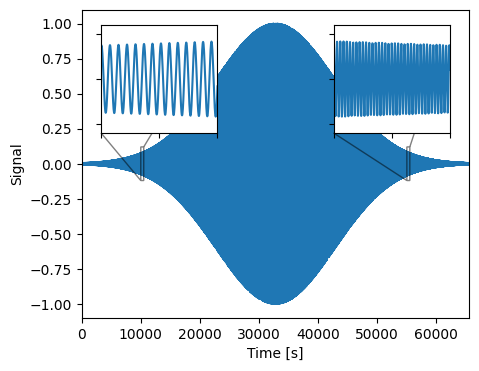
Figure 3 The simple Gaussian wavepacket wavefotm with a frequency that increases linearly with time, as shown by the inset plots.

We can now take the wavelet transform of this signal.

First, we will illustrate the method described above step-by-step; this is shown in Figure 4. For this example we use \(N_{\rm pixels}=5\) (as plotted in Figure 2) and will only interpolate in one dimension on \(f\) (not \(\dot{f}\) or any higher derivatives) using 50 grid points.

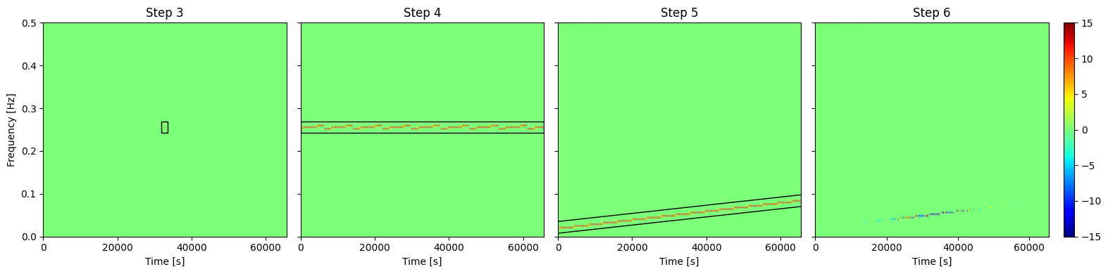
Figure 4 Illustration of the steps involved in the fast wavelet transform. The first panel shows the \(N_{\rm pixels}=5\) interpolated coefficients \(c_{\mathcal{N},m}(F_n)\) in step 3 of the transform, these are highlighted by the black rectangle. There are also interpolated values for the \(s_{\mathcal{N},m}(F_n)\), \(\hat{c}_{\mathcal{N},m}(F_n)\) and \(\hat{s}_{\mathcal{N},m}(F_n)\) coefficients which are not shown. The second panel shows the non-zero \(c_{nm}(F_n)\) coefficients obtained in step 4, these are obtained simply by copying the coefficients obtained in the previous step horizontally in this diagram. The third panel shows the \(c_{nm}(f_n)\) coefficients obtained in step 5, these are obtained simply by translating the coefficients obtained in the previous step vertically in this diagram by an amount \(z_n\). The final panel the wavelet coefficients \(w_{nm}\) obtained in step 6 which include the scaling by the waveform amplitude.

Figure 5 shows a comparison of the wavelet transform computed by the fast method described here (left panel) and computed exactly using the discrete wavelet transform (right panel). These two signals agree well enough that the differences are not visible in this plot (the white-noise mismatch between these two signals is \(8.5\times 10^{-3}\)).

The fast transform is indeed fast. On this toy example using small arrays, the fast transform (left panel Figure 5) takes \(\sim 2\,\mathrm{ms}\) to evaluate on my laptop using a jitted jax implementation which is a factor \(\sim 3\) faster than computing the discrete wavelet transform numerically right panel Figure 5). The speed up should be more significant for the longer and more complicated waveforms common in LISA data analysis.

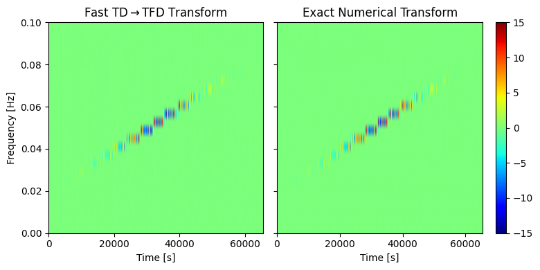
Figure 5 Demonstration of the fast TD \(\rightarrow\) TFD wavelet transform. There are no visible differences between these two plots; the white-noise mismatch between these two signals is \(8.5\times 10^{-3}\).

Finally, just for the sake of visualisation, it is nice to be able to take an inverse discrete wavelet transform to recover the original time-domain signal. This is shown in the Figure 6.

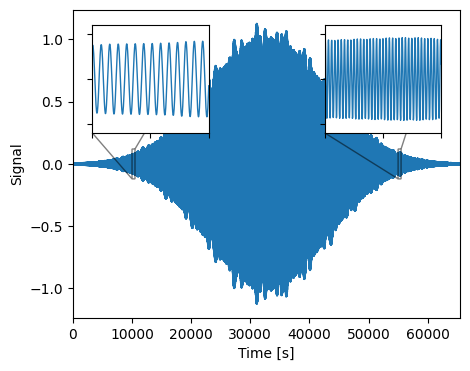
Figure 6 The reconstructed TD signal; the white-noise mismatch with the original signal shown above is \(8.5\times 10^{-3}\).

The small differences between this an the original signal (those responsible for the \(8.5\times 10^{-3}\) mismatch) are due to the approximations made by the fast forward transform: (i) the linear frequency interpolation using just 50 grid points, (ii) neglecting to interpolate in any higher frequency derivatives, (iii) approximating the amplitude as constant across each wavelet duration, (iv) keeping only the loudest \(N_{\rm pixel}=5\) coefficients at each \(n\), (v) neglecting the edge effects at small or large values of the \(n\) index, or (vi) neglecting the zero and Nyquist components of the signal in the \(m=0\) wavelet coefficients. In this example, the dominant source of error comes from (ii); repeating this example while also interpolating over \(\dot{f}\) in the range \((-1.5\times 10^{-6}, 1.5\times 10^{-6})\,\mathrm{Hz}\,\mathrm{s}^{-1}\) using just 3 grid points along this new dimension improves the mismatch by more than an order of magnitude to \(1.5\times 10^{-4}\) (see Figure 7).

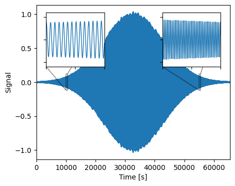
Figure 7 Same as Figure 6 when also interpolating over \(\dot{f}\), in this case the mismatch improves to \(1.5\times 10^{-4}\).

Fast Wavelet Transform (FD \(\rightarrow\) TFD)

Suppose the waveform model is defined in the FD in terms of its amplitude \(A(f)\) and phase \(\Phi(f)\),

(22)\[\tilde{h}(f) = \tilde{h}^+(f)-i\tilde{h}^\times(f) = A(f) \exp\big(i \Phi(f)\big) ,\]

where the amplitude and phase derivative \(\mathrm{d}\Phi/\mathrm{d}f\) change slowly with frequency; i.e.they change by a small amount over the wavelet resolution \(\Delta F\). Generally, a waveform may contain a sum of harmonics of this form. This is what is meant by a “harmonic-based” FD waveform.

The fast FD \(\rightarrow\) TDF transform is conceptually similar to the FD \(\rightarrow\) TDF transform described in the above section except that we expand the phase in frequency. The relationship between the two fast transforms is nicely captured by the diagram in Figure 8.

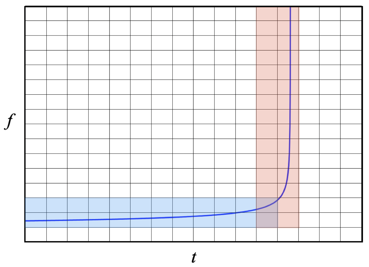
Figure 8 Illustration of the time-frequency decomposition of a waveform harmonic. The horizontal (blue) shaded region indicates where the fast TD \(\rightarrow\) TFD transform is applicable, while the vertical (red) region indicates where the fast FD \(\rightarrow\) TFD transform is applicable. Diagram reproduced from Ref. [2].

SO FAR I HAVE ONLY IMPLEMENTED THE TRANSFORM FROM THE TIME DOMAIN. THIS FD ONE IS COMING NEXT. WATCH THIS SPACE!

References

[1] (1,2)

V. Necula, S. Klimenko & G. Mitselmakher, Transient analysis with fast Wilson-Daubechies time-frequency transform, Journal of Physics: Conference Series 363 012032, 2012. DOI 10.1088/1742-6596/363/1/012032

[2] (1,2)

N. J. Cornish, Time-Frequency Analysis of Gravitational Wave Data, Physical Review D 102 124038, 2020. arXiv:2009.00043

Appendices

Appendix A: Derivation of Time-Shift Properties

Starting from the integral definitions of the \(c_{nm}\) and \(s_{nm}\) coefficients in Eqs.10 and 11, and their corresponding duals, and evaluating these at \(m=0\) gives

(23)\[c_{0m}(f,\dot{f},\ldots) = \int_{-\infty}^{\infty}\mathrm{d}t\; \cos X_0(f,\dot{f},\ldots) g_{0m}(t) ,\]

(24)\[s_{0m}(f,\dot{f},\ldots) = \int_{-\infty}^{\infty}\mathrm{d}t\; \sin X_0(f,\dot{f},\ldots) g_{0m}(t),\]

(25)\[\hat{c}_{0m}(f,\dot{f},\ldots) = \int_{-\infty}^{\infty}\mathrm{d}t\; \cos X_0(f,\dot{f},\ldots) \hat{g}_{0m}(t) ,\]

(26)\[\hat{s}_{0m}(f,\dot{f},\ldots) = \int_{-\infty}^{\infty}\mathrm{d}t\; \sin X_0(f,\dot{f},\ldots) \hat{g}_{0m}(t).\]

Changing the integration variable to \(t'=t+n\Delta T\) (and dropping the prime on \(t\)) gives

(27)\[c_{0m}(f,\dot{f},\ldots) = \int_{-\infty}^{\infty}\mathrm{d}t\; \cos X_n(f,\dot{f},\ldots) g_{0m}(t-n\Delta T) ,\]

(28)\[s_{0m}(f,\dot{f},\ldots) = \int_{-\infty}^{\infty}\mathrm{d}t\; \sin X_n(f,\dot{f},\ldots) g_{0m}(t-n\Delta T),\]

(29)\[\hat{c}_{0m}(f,\dot{f},\ldots) = \int_{-\infty}^{\infty}\mathrm{d}t\; \cos X_n(f,\dot{f},\ldots) \hat{g}_{0m}(t-n\Delta T) ,\]

(30)\[\hat{s}_{0m}(f,\dot{f},\ldots) = \int_{-\infty}^{\infty}\mathrm{d}t\; \sin X_n(f,\dot{f},\ldots) \hat{g}_{0m}(t-n\Delta T).\]

Using the following time-translation property of the basis wavelets (these follow directly from the definitions of the wavelet basis functions and their duals in Eqs.1 and 2)

(31)\[\begin{split}g_{0m}(t-n\Delta T) = \begin{cases} g_{nm}(t) & \mathrm{if}\;n\;\mathrm{is}\;\mathrm{even} \\ \hat{g}_{nm}(t) & \mathrm{if}\;n\;\mathrm{is}\;\mathrm{odd} \end{cases} ,\end{split}\]

(32)\[\begin{split}\hat{g}_{0m}(t-n\Delta T) = \begin{cases} \hat{g}_{nm}(t) & \mathrm{if}\;n\;\mathrm{is}\;\mathrm{even} \\ g_{nm}(t) & \mathrm{if}\;n\;\mathrm{is}\;\mathrm{odd} \end{cases} ,\end{split}\]

gives

(33)\[\begin{split}c_{0m}(f, \dot{f},\ldots) = \begin{cases} c_{nm}(f, \dot{f},\ldots) & \mathrm{if}\;n\;\mathrm{is}\;\mathrm{even} \\ \hat{c}_{nm}(f, \dot{f},\ldots) & \mathrm{if}\;n\;\mathrm{is}\;\mathrm{odd} \end{cases} ,\end{split}\]

(34)\[\begin{split}s_{0m}(f, \dot{f},\ldots) = \begin{cases} s_{nm}(f, \dot{f},\ldots) & \mathrm{if}\;n\;\mathrm{is}\;\mathrm{even} \\ \hat{s}_{nm}(f, \dot{f},\ldots) & \mathrm{if}\;n\;\mathrm{is}\;\mathrm{odd} \end{cases} ,\end{split}\]

(35)\[\begin{split}\hat{c}_{0m}(f, \dot{f},\ldots) = \begin{cases} \hat{c}_{nm}(f, \dot{f},\ldots) & \mathrm{if}\;n\;\mathrm{is}\;\mathrm{even} \\ c_{nm}(f, \dot{f},\ldots) & \mathrm{if}\;n\;\mathrm{is}\;\mathrm{odd} \end{cases} ,\end{split}\]

(36)\[\begin{split}\hat{s}_{0m}(f, \dot{f},\ldots) = \begin{cases} \hat{s}_{nm}(f, \dot{f},\ldots) & \mathrm{if}\;n\;\mathrm{is}\;\mathrm{even} \\ s_{nm}(f, \dot{f},\ldots) & \mathrm{if}\;n\;\mathrm{is}\;\mathrm{odd} \end{cases} .\end{split}\]

Inverting these expressions to find \(c_{nm}\) and \(s_{nm}\) gives

(37)\[\begin{split}c_{nm}(f, \dot{f},\ldots) = \begin{cases} c_{0m}(f, \dot{f},\ldots) & \mathrm{if}\;n\;\mathrm{is}\;\mathrm{even} \\ \hat{c}_{0m}(f, \dot{f},\ldots) & \mathrm{if}\;n\;\mathrm{is}\;\mathrm{odd} \end{cases} ,\end{split}\]

(38)\[\begin{split}s_{nm}(f, \dot{f},\ldots) = \begin{cases} s_{0m}(f, \dot{f},\ldots) & \mathrm{if}\;n\;\mathrm{is}\;\mathrm{even} \\ \hat{s}_{0m}(f, \dot{f},\ldots) & \mathrm{if}\;n\;\mathrm{is}\;\mathrm{odd} \end{cases} .\end{split}\]

Finally, because we have shown that the coefficient only depend on the parity of the index \(n\), we can replace \(n=0\) in these expressions with any other even integer \(\mathcal{N}\). This gives the results in Eqs.13 and 14 of the main text;

(39)\[\begin{split}c_{nm}(f, \dot{f},\ldots) &= \begin{cases} c_{\mathcal{N}m}(f, \dot{f},\ldots) & \mathrm{if}\;n\;\mathrm{is}\;\mathrm{even} \\ \hat{c}_{\mathcal{N}m}(f, \dot{f},\ldots) & \mathrm{if}\;n\;\mathrm{is}\;\mathrm{odd} \end{cases} ,\end{split}\]

(40)\[\begin{split}s_{nm}(f, \dot{f},\ldots) &= \begin{cases} s_{\mathcal{N}m}(f, \dot{f},\ldots) & \mathrm{if}\;n\;\mathrm{is}\;\mathrm{even} \\ \hat{s}_{\mathcal{N}m}(f, \dot{f},\ldots) & \mathrm{if}\;n\;\mathrm{is}\;\mathrm{odd} \end{cases} .\end{split}\]

Note that these results do not hold precisely for the discrete wavelet transform (i.e. if the integrals over \(t\) are replaced with finite sums) for values of \(n\) near the beginning and end of the allowed range. This is discussed in more detail in the main text.

Appendix B: Derivation of Freq-Shift Properties

Start from the definitions of the \(c_{nm}\) and \(s_{nm}\) coefficients in Eqs.10 and 11, shift by an even multiple of the wavelet frequency resolution; \(f\rightarrow f+2z\Delta F\).

(41)\[c_{nm}(f+z\Delta F) = \int\mathrm{d}t\;\cos\big(X_n(f)+4\pi z[t-t_n] \Delta F\big)g_{nm}(t)\]

(42)\[s_{nm}(f+z\Delta F) = \int\mathrm{d}t\;\sin\big(X_n(f)+4\pi z[t-t_n] \Delta F\big)g_{nm}(t)\]

Throughout this appendix, we will simplify our notation by assuming that all quantities like \(c_{nm}(f, \dot{f}, \ldots)\), \(s_{nm}(f, \dot{f}, \ldots)\), and \(X_{n}(f, \dot{f}, \ldots)\) depend only on the frequency \(f\) and suppress any dependence on higher derivatives of the phase in our notation. This will not effect any of our conclusions.

We now consider the cases of odd and even \(n+m\) separately.

CASE #1: \(n+m\) EVEN

Substituting the wavelet definition into the expressions for the shifted coefficients gives

(43)\[c_{nm}(f+2z\Delta F) = \sqrt{2} \int\mathrm{d}t\; \cos\big(X_n(f)+4\pi z [t-n\Delta T] \Delta F\big) \cos\big(2\pi m [t-n\Delta T] \Delta F\big) \phi(t-n\Delta T),\]

(44)\[s_{nm}(f+2z\Delta F) = \sqrt{2} \int\mathrm{d}t\; \sin\big(X_n(f)+4\pi z [t-n\Delta T] \Delta F\big) \cos\big(2\pi m [t-n\Delta T] \Delta F\big) \phi(t-n\Delta T).\]

Using the compound angle trigonometric formulae and separating terms this becomes

(45)\[\begin{split}c_{nm}(f+2z\Delta F) = \sqrt{2} \int\mathrm{d}t\; \cos X_n(f) \cos\big(4\pi z [t-n\Delta T] \Delta F\big) \cos\big(2\pi m[t-n\Delta T]\Delta F\big) \phi(t-n\Delta T) \nonumber \\ - \sqrt{2} \int\mathrm{d}t\; \sin X_n(f) \sin\big(4\pi z [t-n\Delta T] \Delta F\big) \cos\big(2\pi m [t-n\Delta T] \Delta F\big) \phi(t-n\Delta T),\end{split}\]

(46)\[\begin{split}s_{nm}(f+2z\Delta F) = \sqrt{2} \int\mathrm{d}t\; \cos X_n(f) \sin\big(4\pi z [t-n\Delta T] \Delta F\big) \cos\big(2\pi m[t-n\Delta T]\Delta F\big) \phi(t-n\Delta T) \nonumber \\ + \sqrt{2} \int\mathrm{d}t\; \sin X_n(f) \cos\big(4\pi z [t-n\Delta T] \Delta F\big) \cos\big(2\pi m[t-n\Delta T]\Delta F\big) \phi(t-n\Delta T).\end{split}\]

Using the trig identities \(\cos A \cos B = \frac{1}{2}\big(\cos[A-B]+\cos[A+B]\big)`\) and \(\sin A \cos B = \frac{1}{2}\big(\sin[A-B]+\sin[A+B]\big)\) this becomes

(47)\[\begin{split}c_{nm}(f+2z\Delta F) = \frac{1}{\sqrt{2}} \int\mathrm{d}t\; \cos X_n(f) \cos\big(2\pi[m-2z][t-n\Delta T]\Delta F\big) \phi(t-n\Delta T) \\ +\frac{1}{\sqrt{2}} \int\mathrm{d}t\; \cos X_n(f) \cos\big(2\pi[m+2z][t-n\Delta T]\Delta F\big) \phi(t-n\Delta T) \\ +\frac{1}{\sqrt{2}} \int\mathrm{d}t\; \sin X_n(f) \sin\big(2\pi[m-2z][t-n\Delta T]\Delta F\big) \phi(t-n\Delta T) \\ -\frac{1}{\sqrt{2}} \int\mathrm{d}t\; \sin X_n(f) \sin\big(2\pi[m+2z][t-n\Delta T]\Delta F\big) \phi(t-n\Delta T) , \\\end{split}\]

(48)\[\begin{split}s_{nm}(f+2z\Delta F) = \frac{-1}{\sqrt{2}} \int\mathrm{d}t\; \cos X_n(f) \sin\big(2\pi[m-2z][t-n\Delta T]\Delta F\big) \phi(t-n\Delta T) \\ +\frac{1}{\sqrt{2}} \int\mathrm{d}t\; \cos X_n(f) \sin\big(2\pi[m+2z][t-n\Delta T]\Delta F\big) \phi(t-n\Delta T) \\ +\frac{1}{\sqrt{2}} \int\mathrm{d}t\; \sin X_n(f) \cos\big(2\pi[m-2z][t-n\Delta T]\Delta F\big) \phi(t-n\Delta T) \\ +\frac{1}{\sqrt{2}} \int\mathrm{d}t\; \sin X_n(f) \cos\big(2\pi[m+2z][t-n\Delta T]\Delta F\big) \phi(t-n\Delta T) .\end{split}\]

Finally, using the definitions of \(g_{nm}\), \(c_{nm}\), and \(s_{nm}\) (and their dual equivalents), this simplifies to a result involving the coefficients evaluated at frequency \(f\);

(49)\[c_{nm}(f+2z\Delta F) = \frac{1}{2} \Big( c_{n(m-2z)}(f) + c_{n(m+2z)}(f) + \hat{s}_{n(m-2z)}(f) - \hat{s}_{n(m+2z)}(f) \Big) ,\]

(50)\[s_{nm}(f+2z\Delta F) = \frac{1}{2} \Big( s_{n(m-2z)}(f)+s_{n(m+2z)}(f) - \hat{c}_{n(m-2z)}(f) + \hat{c}_{n(m+2z)}(f) \Big) .\]

Note that this is that step that requires the frequency shift to be an even multiple of \(\Delta F\); this is needed because if \(n+m\) is even then so is \(n+m\pm 2z\) and we can still use the same case in the wavelet definition.

CASE #1: \(n+m\) ODD

An identical procedure in this case gives

(51)\[c_{nm}(f+2z\Delta F) = \frac{1}{2} \Big( c_{n(m-2z)}(f) + c_{n(m+2z)}(f) - \hat{s}_{n(m-2z)}(f) + \hat{s}_{n(m+2z)}(f) \Big) ,\]

(52)\[s_{nm}(f+2z\Delta F) = \frac{1}{2} \Big( s_{n(m-2z)}(f) + s_{n(m+2z)}(f) + \hat{c}_{n(m-2z)}(f) - \hat{c}_{n(m+2z)}(f) \Big) .\]

The final step involves taking care of the differing signs in these equations by inserting appropriate factors of \((-1)^{n+m}\). This gives the results in Eqs.15 and 16 valid for all \(n\) and \(m\).